DTW (Xp,Y q) = KDTW xy(X
p,Y q) + KDTW xx(X
p,Y q) DTW (Xp,Y q) = KDTW xy(X
p,Y q) + KDTW xx(X
p,Y q) |
where |
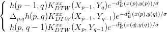
KDTW xy(X
p,Y q) = β ⋅ e-dE2(x(p),y(q))∕σ |
∑
 |
and |
KDTW xx(X
p,Y q) = β⋅ |
∑
 |
We introduce in this short presentation a regularized version of the Dynamic Time Warping (DTW) distance, that we call KDTW . KDTW is in fact a similarity measure constructed from DTW with the property that KDTW (.,.) is a positive definite kernel (homogeneous to an inner product in the so-called Reproducing Kernel Hilbert Space). Following earlier work by Cuturi & al. [1], namely the so-called Global Alignment kernel (GA-kernel), the derivation of KDTW is detailed in Marteau & Gibet 2014 [4]. KDTW is a convolution kernel as defined in [2]. After giving a recursive definition of KDTW , we present hereinafter a small experiment to highlight the benefit of a positive definite time elastic kernel to process time series data. Some code is provided (as is) by the end of the presentation to make it easier to reproduce some of our results.
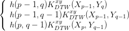
The recursive definition of KDTW kernel as defined in [4] is as follows:
| (1) |
 . If σ tends to 0 (is small comparatively to the
variance of the time series samples) then β will have to tend to 1. By
default, β =
. If σ tends to 0 (is small comparatively to the
variance of the time series samples) then β will have to tend to 1. By
default, β =  , which prevents the "infinity explosion" of the kernel.
The recursive definition given above shows that the algorithmic complexity of KDTW is O(N2), where N is the length of the longest of the two time series given in entry, and when no corridor size is specified. This complexity drop down to O(C.N) when a symmetric corridor of size C is exploited.
The main idea leading to the construction of positive definite kernels from a given elastic distance used to match two time series is simply the following: instead of keeping only one of the best alignment paths, the new kernel will try to sum up the costs of all the existing sub-sequence alignment paths with some weighting factor that will favor good alignments while penalizing bad alignments. In addition, this weighting factor can be optimized. Thus, basically we replace the min (or max) operator by a summation operator and introduce a symmetric corridor function (the function h in the recursive equation above) to optionally limit the summation and the computational cost. Then we add a regularizing recursive term (Kxx) such that the proof of the positive definiteness property can be understood as a direct consequence of the Haussler’s convolution theorem [2]. Please see [4] for more details.
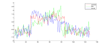
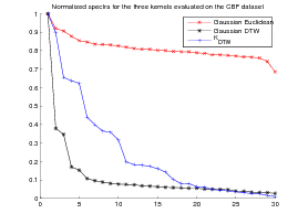
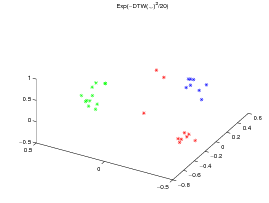
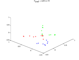
For the first experiment we use the Cylinder(C) Bell(B) Funel(F) TRAIN data set as available at the UCR Time Series Classification-Clustering Datasets repository [3]. The dataset contains 30 time series which belong to the three categories (C, B, F) and take the forms presented in figure 1.
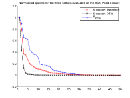
The second experiment concerns the Gun_Point TRAIN dataset that also belongs to the UCR time series dataset repository. It contains two classes and 50 time series. For more details please see [3].
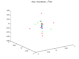
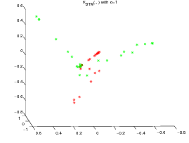
For the two datasets, a KPCA [5] is performed respectively on the normalized exp(-dE(.,.)2∕20) kernel matrix (left subfigure, where d E stands for the Euclidean distance), the exp(-DTW(.,.)2∕20) kernel matrix (center subfigure) and the KDTW (.,.) kernel matrix (right subfigure, with σ = 15 for the CBF dataset and σ = 1 for the Gun_Point dataset). The Gaussian like kernel is not required for KDTW since it is somehow already in use into the computation of the local kernels (c.f. the definition above).
All the times series are then projected on the first three eigen vectors obtained by KPCA as presented on figures 2 and 3.
   |
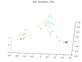 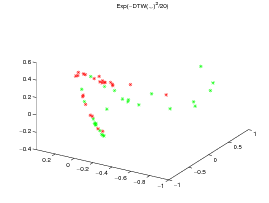  |
Note that, although the DTW(.,.) matrix is not definite in general, exp(DTW(.,.)2∕20 matrix is definite on the CBF dataset but not on the Gun_Point dataset. This may explain the good clustering obtained by the Gaussian DTW kernel on CBF data set and its drawback on the Gun_Point dataset for which KPCA is not well funded. By contrast, these gram matrices are always positive definite for the Euclidean and KDTW kernels. Figure 4 presents the normalized spectra of the gram matrices for these kernels to give some highlighting about the dimensionality reduction that can be achieved with each kernel while maintaining a good separability between the classes.
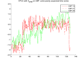
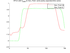
The experiment shows that, although The DTW Gaussian kernel works particularly well on the CBF dataset, KDTW achieves a better natural clustering in average than the Euclidean or DTW Gaussian kernels. KDTW seems to act as a compromise between Euclidean Distance and DTW distance substituting Gaussian kernel. Figure 5 below shows some time series belonging to different classes that are poorly separated by the KDTW kernel. For the Gun_Point dataset the two presented instances seem very close. For the CBF dataset this is likely due to a loss of selectivity induced by the summation operator of KDTW .
The Octave/Matlab code (without corridor) for evaluating the KDTW similarity (pd kernel) between two time series is available here.
The Octave/Matlab code (without corridor) used to evaluate the KPCA on the Euclidean distance, DTW and KDTW kernel matrices is available here.
[1] M. Cuturi, J.-P. Vert, Ø. Birkenes, and Tomoko Matsui. A kernel for time series based on global alignments. In Acoustics, Speech and Signal Processing, 2007. ICASSP 2007. IEEE International Conference on, volume 2, pages II–413–II–416, April 2007.
[2] David Haussler. Convolution kernels on discrete structures. Technical Report UCS-CRL-99-10, University of California at Santa Cruz, Santa Cruz, CA, USA, 1999.
[3] E. J. Keogh, X. Xi, L. Wei, and C.A. Ratanamahatana. The UCR time series classification-clustering datasets, 2006. http://wwwcs.ucr.edu/ eamonn/time_series_data/.
[4] Pierre-François Marteau and Sylvie Gibet. On Recursive Edit Distance Kernels with Application to Time Series Classification. IEEE Transactions on Neural Networks and Learning Systems, pages 1–14, June 2014. 14 pages.
[5] Bernhard Schölkopf, Alexander Smola, and Klaus-Robert Müller. Nonlinear component analysis as a kernel eigenvalue problem. Neural Comput., 10(5):1299–1319, July 1998.